How to Build an Algorithmic Trading System with Python

(Based on 3 Years of Fixing Mistakes and Gaining Confidence + Results)

Feb 05, 2025

(Based on 3 Years of Fixing Mistakes and Gaining Confidence + Results)

Algorithmic trading might seem like an advanced game reserved for Wall Street professionals, but with the right approach, anyone with programming skills and a strong understanding of financial markets can build an effective trading system.

After three years of learning, making mistakes, and refining my approach, I now manage a portfolio worth $6,500,000. I’m still learning, but I want to share the key insights that helped me reach this point.

This guide will walk you through the essential steps to build an algorithmic trading system using Python. Let’s get started.

1. Data Sourcing & Quality

A trading algorithm is only as good as the data it relies on. Poor-quality data leads to bad decisions.

Key Steps in Data Preparation:

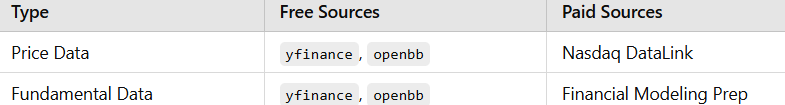
✅ Use reliable financial data sources.
✅ Scrub for inconsistencies & missing values.
✅ Consider paid APIs for accuracy in serious trading.

Recommended Data Sources

Example: Fetching Data with `yfinance`

Here’s how you can pull stock price data using yfinance:

import yfinance as yf  

# Fetch historical data for AAPL
df = yf.download("AAPL", start="2022-01-01", end="2023-01-01", auto_adjust=True)

# Check if data was successfully retrieved
if df.empty:
    print("Failed to fetch data. Please check ticker or date range.")
else:
    print(df.head())  # Display first few rows

👉 For serious trading, consider paid APIs to avoid limitations and get institutional-quality data.

2. Alpha Model (Generating Buy/Sell Signals)

This is the brain of your strategy — it decides when to buy or sell.

Types of Trading Strategies

📌 Mean Reversion — Buy when prices dip below average, sell when they rise above.
📌 Trend Following — Ride the trend (buy in uptrends, sell in downtrends).
📌 Machine Learning-Based — Use AI models to predict price movements.

Example: Simple Moving Average (SMA) Strategy

We’ll use a basic crossover strategy:
✅ Buy when the short-term SMA crosses above the long-term SMA.
✅ Sell when the short-term SMA crosses below the long-term SMA.

import pandas as pd
import numpy as np

# Example: Load data (Ensure df is defined)
# df = pd.read_csv("your_data.csv")  # Uncomment if needed

# Ensure the DataFrame has a 'Close' column
if "Close" in df.columns:
    # Calculate moving averages
    df["SMA_50"] = df["Close"].rolling(window=50, min_periods=1).mean()
    df["SMA_200"] = df["Close"].rolling(window=200, min_periods=1).mean()
    
    # Define buy/sell signals
    df["Signal"] = np.where(df["SMA_50"] > df["SMA_200"], 1, 0)
    
    # Display the last few rows
    print(df[["Close", "SMA_50", "SMA_200", "Signal"]].tail())
else:
    print("Error: 'Close' column not found in DataFrame.")

👉 You can enhance this with more indicators or machine learning techniques.

3. Portfolio Construction

Once you have trade signals, you need to allocate capital efficiently across different stocks.

Common Portfolio Allocation Methods

📌 Equal-weighted — Each asset gets the same investment.
📌 Risk-parity — Allocate based on risk levels.
📌 Optimized weighting — Use algorithms like Markowitz’s Modern Portfolio Theory.

Example: Risk-Parity Portfolio using `Riskfolio-Lib`

import pandas as pd
import riskfolio as rp

# Assume `returns` is a pandas DataFrame with historical stock returns
# Ensure `returns` is properly defined before running the code
if 'returns' not in locals():
    raise ValueError("The variable 'returns' must be a pandas DataFrame containing historical returns.")

# Initialize Portfolio object
port = rp.Portfolio(returns=returns)

# Compute assets statistics (mean, covariance, etc.)
port.assets_stats(method_mu='hist', method_cov='hist')

# Perform risk-parity optimization (Minimum Variance)
weights = port.rp_optimization(model='Classic', rm='MV', obj='MinRisk', hist=True)

# Display the portfolio weights
print(weights)

👉 Start simple, then optimize as you learn more about risk management.

4. Transaction Costs & Execution

Even a profitable strategy can fail if you ignore slippage, commissions, and order types.

Key Considerations:

✅ Simulate execution costs in backtests.
✅ Use realistic order types (market, limit, stop-loss).
✅ Optimize trade execution to avoid price impact.

Example: Incorporating Slippage in Backtesting (`VectorBT`)

import vectorbt as vbt  

# Assuming df["Signal"] contains 1 for long, -1 for short, and 0 for no position
entries = df["Signal"] > 0  # Enter long when signal is 1
exits = df["Signal"] < 0  # Exit when signal is -1

# Simulate a backtest with slippage & fees
portfolio = vbt.Portfolio.from_signals(
    close=df["Close"],
    entries=entries,
    exits=exits,
    size=100,
    fees=0.001,  # 0.1% fees per trade
    slippage=0.005  # 0.5% slippage
)

# Print portfolio performance
print(portfolio.performance())

👉 Always factor in real-world execution issues when designing strategies.

5. Risk Management

Risk management ensures you survive market downturns and don’t blow up your account.

Risk Control Techniques:

📌 Stop-loss & trailing stops — Limit potential losses.
📌 Position sizing — Adjust trade size based on volatility.
📌 Drawdown monitoring — Track portfolio declines.

Example: Visualizing Drawdowns with `Plotly`

import pandas as pd
import plotly.graph_objects as go  

# Sample Data (Ensure df is defined in your context)
# df = pd.read_csv("your_data.csv", parse_dates=["Date"], index_col="Date")

df["Drawdown"] = df["Close"] / df["Close"].cummax() - 1

# Create Figure
fig = go.Figure()

# Add Drawdown Plot
fig.add_trace(go.Scatter(
    x=df.index, 
    y=df["Drawdown"], 
    fill='tozeroy', 
    mode='lines',  # Ensure line chart
    name="Drawdown"
))

# Layout Enhancements
fig.update_layout(
    title="Drawdown Chart",
    xaxis_title="Date",
    yaxis_title="Drawdown",
    template="plotly_white"
)

# Show Figure
fig.show()

👉 Monitoring drawdowns helps you adjust risk dynamically.

6. Putting It All Together

Now let’s outline the complete trading pipeline:

1️⃣ Data Ingestion — Fetch & clean financial data.
2️⃣ Alpha Model — Generate trade signals.
3️⃣ Portfolio Construction — Allocate capital wisely.
4️⃣ Execution — Optimize orders & minimize costs.
5️⃣ Risk Management — Monitor losses & adjust risk dynamically.

Modular Trading System in Python

import numpy as np
import pandas as pd
import yfinance as yf

class TradingSystem:
    def __init__(self, data):
        self.data = data

    def generate_signals(self):
        self.data["SMA_50"] = self.data["Close"].rolling(window=50).mean()
        self.data["SMA_200"] = self.data["Close"].rolling(window=200).mean()
        self.data["Signal"] = np.where(self.data["SMA_50"] > self.data["SMA_200"], 1, 0)

    def backtest(self):
        self.data["Returns"] = self.data["Close"].pct_change() * self.data["Signal"].shift(1)
        return self.data["Returns"].cumsum()

# Load data
df = yf.download("AAPL", start="2022-01-01", end="2023-01-01")

# Run strategy
trading_system = TradingSystem(df)
trading_system.generate_signals()
performance = trading_system.backtest()

# Print last 5 values of performance
print(performance.tail())

Overfitting in Algorithmic Trading

Overfitting occurs when a trading algorithm is excessively tailored to historical data, capturing noise rather than the underlying market patterns. This results in impressive backtest performance but poor real-world results, as the model fails to generalize to new, unseen data.

Solution: Implementing Robust Validation Techniques

To mitigate overfitting, it’s essential to employ rigorous validation methods:

Train-Test Split: Divide your data into separate training and testing sets to evaluate performance on unseen data.
Cross-Validation: Use techniques like k-fold cross-validation to assess the model’s stability across different data subsets.
Regularization: Apply regularization methods to prevent the model from becoming too complex and capturing noise.

Implementation in Python

Building upon our previous trading system, we can integrate these validation techniques. Assuming we have a dataset df with historical stock prices, here's how to implement a train-test split and cross-validation:

import pandas as pd
import numpy as np
from sklearn.model_selection import TimeSeriesSplit
from sklearn.metrics import accuracy_score

# Assuming df is your DataFrame with historical data
df = df.copy()  # Avoid modifying the original DataFrame

# Feature engineering: Calculate moving averages
df['SMA_50'] = df['Close'].rolling(window=50, min_periods=1).mean()
df['SMA_200'] = df['Close'].rolling(window=200, min_periods=1).mean()

# Drop rows with NaN values
df.dropna(inplace=True)

# Define features and target
X = df[['SMA_50', 'SMA_200']]
y = np.where(df['SMA_50'].values > df['SMA_200'].values, 1, 0)  # 1 for buy signal, 0 for sell

# TimeSeriesSplit for cross-validation
tscv = TimeSeriesSplit(n_splits=5)
accuracy_scores = []

for train_index, test_index in tscv.split(X):
    X_train, X_test = X.iloc[train_index], X.iloc[test_index]
    y_train, y_test = y[train_index], y[test_index]  # Ensure proper indexing

    # Simple strategy: Predict based on SMA crossover
    y_pred = np.where(X_test['SMA_50'] > X_test['SMA_200'], 1, 0)

    # Calculate accuracy
    accuracy = accuracy_score(y_test, y_pred)
    accuracy_scores.append(accuracy)

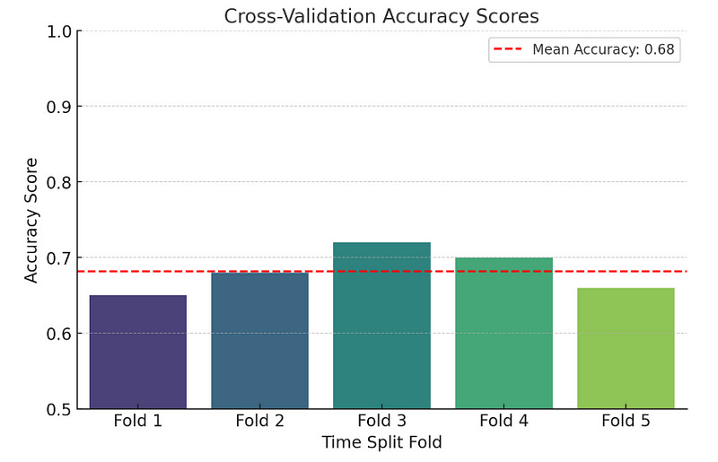
print(f'Cross-Validation Accuracy Scores: {accuracy_scores}')
print(f'Mean Accuracy: {np.mean(accuracy_scores):.4f}')

We calculate the 50-day and 200-day Simple Moving Averages (SMA) to use as features.

Using TimeSeriesSplit from scikit-learn ensures that the training data always precedes the testing data, respecting the temporal order of financial data.

In each split, we predict buy signals where the 50-day SMA is greater than the 200-day SMA and calculate the accuracy of these predictions.

import matplotlib.pyplot as plt
import seaborn as sns
import numpy as np

# Sample accuracy scores (Replace with actual values from your model)
accuracy_scores = [0.65, 0.68, 0.72, 0.70, 0.66]

# Create a bar plot
plt.figure(figsize=(8, 5))
sns.barplot(x=[f"Fold {i+1}" for i in range(len(accuracy_scores))], y=accuracy_scores, palette="viridis")

# Add titles and labels
plt.title("Cross-Validation Accuracy Scores", fontsize=14)
plt.xlabel("Time Split Fold", fontsize=12)
plt.ylabel("Accuracy Score", fontsize=12)
plt.ylim(0.5, 1.0)  # Set y-axis limits for better visualization

# Show the mean accuracy as a horizontal line
mean_accuracy = np.mean(accuracy_scores)
plt.axhline(mean_accuracy, color='red', linestyle='--', label=f"Mean Accuracy: {mean_accuracy:.2f}")
plt.legend()

# Show the plot
plt.show()

✅ Start simple, then iterate.
✅ Use quality data & account for real-world issues.
✅ Backtest rigorously & manage risk properly.

I made a ton of mistakes before getting things right, but persistence pays off.

📌 Want to build a trading system? Start coding today! 🚀

A Message from InsiderFinance

Thanks for being a part of our community! Before you go:

👏 Clap for the story and follow the author 👉
📰 View more content in the InsiderFinance Wire
📚 Take our FREE Masterclass
📈 Discover Powerful Trading Tools

DataScience Nexus

Discussion about this post

Ready for more?