15 Free Quant Trading Strategies in Python

Quantitative trading, commonly used by hedge funds and high-frequency traders, may seem complex,, but at its core, it’s about using data…

Quantitative trading, commonly used by hedge funds and high-frequency traders, may seem complex,, but at its core, it’s about using data and algorithms to make trading decisions. The good news? You don’t need millions of dollars or a PhD in mathematics to get started.

This article introduces 15 free, fully coded quant trading strategies in Python that can help you dive into the world of systematic trading. These strategies range from momentum trading, statistical arbitrage, support & resistance reversals, and options backtesting, among others.

Before we explore some of these strategies, let’s set the stage with two inspiring quotes:

“We’re right 50.75 percent of the time… but we’re 100 percent right 50.75 percent of the time. You can make billions that way.”
 — Robert Mercer, co-CEO of Renaissance Technologies

“If you trade a lot, you only need to be right 51 percent of the time. We need a smaller edge on each trade.”
 — Elwyn Berlekamp, co-founder of Combinatorial Game Theory

These quotes highlight a crucial principle in quant trading: small edges can compound into big profits over time. The key is discipline, strategy, and automation.

Why These Strategies Matter

Most of the strategies in this repository focus on technical indicators and automated trading. They include:
✅ Momentum trading (trading with the trend)
✅ Opening range breakout (capitalizing on market opening moves)
✅ Support & resistance reversals (buying at key levels)
✅ Statistical arbitrage (using math to find mispricings)
✅ Options backtesting (analyzing options strategies over time)

While technical analysis dominates, quant trading isn’t limited to just price patterns. Advanced quants explore areas like:
🔹 Derivative pricing mismatches (finding inefficiencies in options and futures)
🔹 Alternative data for alpha generation (social media, satellite data, etc.)
🔹 Market microstructure and high-frequency execution

Unfortunately, high-frequency trading (HFT) is not included in these strategies due to the high cost of acquiring ultra-low-latency data. However, everything here is historical backtesting and forward testing, primarily done in Python (with potential Julia support in the future).

1. London Breakout — The Power of Market Overlaps

One of the most exciting forex strategies is the London Breakout, an intraday strategy based on opening range breakout trading.

Why Does It Work?

The foreign exchange (FX) market runs 24/7 across different time zones, meaning traders can observe price movements before their local market opens. Tokyo and London are two of the largest FX markets, and this strategy exploits the information flow between them.

How It Works

📌 Key time window: 7:00 AM — 7:59 AM GMT (just before London opens at 8:00 AM GMT).
📌 Setup: Identify the high and low of this time window.
📌 Entry: If price breaks above the high, go long. If it breaks below the low, go short.
📌 Risk management: Use stop losses to avoid false breakouts.

Python Code for London Breakout

Here’s a simple implementation of the London Breakout strategy in Python using Pandas:

import pandas as pd  

# Load historical forex data (assuming a DataFrame with 'Time', 'High', 'Low', 'Close' columns)
df = pd.read_csv("forex_data.csv")  
# Convert time to datetime and filter for London Breakout period
df['Time'] = pd.to_datetime(df['Time'])
london_pre_open = df[(df['Time'].dt.hour == 7)]  
# Define breakout levels
high_threshold = london_pre_open['High'].max()
low_threshold = london_pre_open['Low'].min()
# Trading logic: Check breakout conditions
df['Long'] = (df['High'] > high_threshold)  
df['Short'] = (df['Low'] < low_threshold)
# Display results
print(df[['Time', 'High', 'Low', 'Close', 'Long', 'Short']])

This strategy capitalizes on the information gap between Tokyo’s close and London’s open.

2. Awesome Oscillator — Beating Traditional Indicators

The Awesome Oscillator is a momentum-based trading indicator, an upgraded version of the MACD. It improves upon simple moving averages by using the mean of high and low prices instead of closing prices.

Why Does It Work?

The oscillator helps spot momentum shifts using:
✅ Traditional moving average divergence
✅ Twin Peaks (W-bottom pattern)
✅ Saucer strategy (fast signal response)

Python Code for Awesome Oscillator

Below is a Python implementation of the Awesome Oscillator with the Saucer strategy:

import pandas as pd  

# Load historical data
df = pd.read_csv("forex_data.csv")  
# Calculate Awesome Oscillator (AO)
df['Median Price'] = (df['High'] + df['Low']) / 2  
df['AO'] = df['Median Price'].rolling(window=5).mean() - df['Median Price'].rolling(window=34).mean()  
# Saucer strategy: Buy if AO shows two consecutive upward bars
df['Saucer Buy'] = (df['AO'].shift(2) < df['AO'].shift(1)) & (df['AO'].shift(1) < df['AO'])  
print(df[['Time', 'AO', 'Saucer Buy']])

This allows traders to capture momentum shifts before traditional MACD reacts.

3. Oil Money Project — The Petrocurrency Phenomenon

Ever wondered if oil prices influence the value of oil-exporting nations’ currencies? This strategy explores the relationship between crude oil and petrocurrencies like the Canadian Dollar (CAD), Norwegian Krone (NOK), and Russian Ruble (RUB).

The Hypothesis

Many studies show a correlation between oil prices and petrocurrencies, but correlation does not imply causality. This project attempts to prove causation using data-driven analysis.

How It Works

📌 Collect crude oil price data and petrocurrency exchange rates
📌 Run regression tests to see if oil prices predict currency movements
📌 Backtest trading strategies based on oil price trends

Python Code for Oil Money Correlation

import pandas as pd
import statsmodels.api as sm  

# Load oil price and forex data
oil_data = pd.read_csv("oil_prices.csv")  
fx_data = pd.read_csv("forex_rates.csv")  
# Merge datasets on date
df = pd.merge(oil_data, fx_data, on="Date")  
# Run regression: Does oil price predict currency moves?
X = sm.add_constant(df['Oil Price'])
y = df['CAD/USD']
model = sm.OLS(y, X).fit()  
print(model.summary())

This statistical approach quantifies the relationship between oil prices and petrocurrencies, offering insights into potential trades.

4. MACD Oscillator

Concept: The Moving Average Convergence/Divergence (MACD) is a classic momentum indicator that helps identify trends.

How It Works:

• Compute a short-term moving average (e.g., 12-day EMA) and a long-term moving average (e.g., 26-day EMA).

• The MACD line is the difference between the two EMAs.

• When the MACD line crosses above the signal line (9-day EMA of MACD), it’s a buy signal.

• When it crosses below, it’s a sell signal.

Python Code:

import pandas as pd
import numpy as np
import matplotlib.pyplot as plt

def macd_strategy(data, short_window=12, long_window=26, signal_window=9):
    data['ShortEMA'] = data['Close'].ewm(span=short_window, adjust=False).mean()
    data['LongEMA'] = data['Close'].ewm(span=long_window, adjust=False).mean()
    data['MACD'] = data['ShortEMA'] - data['LongEMA']
    data['Signal'] = data['MACD'].ewm(span=signal_window, adjust=False).mean()
    
    data['Buy'] = (data['MACD'] > data['Signal'])  
    data['Sell'] = (data['MACD'] < data['Signal'])  
    return data
# Example usage
data = pd.read_csv('stock_data.csv')  # Replace with your dataset
data = macd_strategy(data)

5. Pair Trading (Statistical Arbitrage)

Concept: This strategy identifies two cointegrated stocks (stocks that move together) and trades when they diverge.

How It Works:

• Find two correlated stocks (e.g., Coca-Cola and Pepsi).

• Use the Engle-Granger test to check for cointegration.

• If the price spread widens, buy the cheaper stock and short the expensive one.

• Close the trade when they revert to the mean.

Python Code:

from statsmodels.tsa.stattools import coint
import numpy as np


def check_cointegration(stock1, stock2):
    score, p_value, _ = coint(stock1, stock2)
    return p_value  # p-value < 0.05 indicates cointegration
# Example usage
stock1 = np.random.normal(0, 1, 100)  # Replace with actual stock prices
stock2 = stock1 + np.random.normal(0, 0.1, 100)  
print("P-value:", check_cointegration(stock1, stock2))

6. Heikin-Ashi Candlestick

Concept: A modified candlestick chart that reduces market noise.

How It Works:

• Compute Heikin-Ashi open, close, high, and low prices.

• Identify trends more clearly compared to regular candlestick charts.

Python Code:

def heikin_ashi(data):
    ha_data = data.copy()
    ha_data['HA_Close'] = (data['Open'] + data['High'] + data['Low'] + data['Close']) / 4
    ha_data['HA_Open'] = (data['Open'].shift(1) + data['Close'].shift(1)) / 2
    ha_data['HA_High'] = data[['High', 'HA_Open', 'HA_Close']].max(axis=1)
    ha_data['HA_Low'] = data[['Low', 'HA_Open', 'HA_Close']].min(axis=1)
    return ha_data

7. Dual Thrust Strategy

📌 A simple opening range breakout strategy

If you Google Dual Thrust, you might end up reading about rocket engines. But don’t worry, this strategy has nothing to do with space travel! Instead, it’s a momentum-based trading strategy that identifies breakout opportunities.

How It Works

• Calculate upper and lower thresholds based on previous days’ open, close, high, and low prices.

• When the price exceeds the upper threshold, take a long position.

• When the price drops below the lower threshold, take a short position.

• If the price moves from one threshold to another, reverse the position.

• Close all positions by the end of the day.

💡 It’s a great strategy for intraday trading but lacks stop-loss measures. Be sure to manage risk properly.

Python Code for Dual Thrust

import pandas as pd

# Load historical data
data = pd.read_csv("market_data.csv")
# Define K values (these should be optimized based on asset and timeframe)
K1 = 0.5
K2 = 0.5
# Calculate thresholds
high_low_range = data["High"] - data["Low"]
high_close_range = abs(data["High"] - data["Close"].shift(1))
low_close_range = abs(data["Low"] - data["Close"].shift(1))
HH = data["High"].rolling(10).max()
LL = data["Low"].rolling(10).min()
UPPER_THRESHOLD = data["Open"] + K1 * (HH - LL)
LOWER_THRESHOLD = data["Open"] - K2 * (HH - LL)
# Trading signals
data["Signal"] = 0
data.loc[data["Close"] > UPPER_THRESHOLD, "Signal"] = 1
data.loc[data["Close"] < LOWER_THRESHOLD, "Signal"] = -1
print(data[["Date", "Close", "Signal"]].tail())

8. Parabolic SAR Strategy

📌 A trend-following strategy using stop and reverse signals

Parabolic SAR (Stop And Reverse) is a popular technical indicator that helps determine trend direction and potential reversal points. Developed by Welles Wilder, it places dotted markers above or below price movements:
✅ If dots are below price → Uptrend
❌ If dots are above price → Downtrend

How It Works

• Calculate Parabolic SAR values.

• If SAR crosses above the price, take a short position.

• If SAR crosses below the price, take a long position.

• Adjust stop-loss dynamically based on SAR values.

Python Code for Parabolic SAR

import talib

# Load market data
data["SAR"] = talib.SAR(data["High"], data["Low"], acceleration=0.02, maximum=0.2)
# Trading signals
data["Signal"] = 0
data.loc[data["Close"] > data["SAR"], "Signal"] = 1  # Buy
data.loc[data["Close"] < data["SAR"], "Signal"] = -1  # Sell
print(data[["Date", "Close", "SAR", "Signal"]].tail())

🔎 SAR can be tricky to implement due to its recursive nature. Consider tuning acceleration and max step parameters for better results.

9. Bollinger Bands Pattern Recognition

📌 A volatility-based strategy that adapts to market conditions

Bollinger Bands consist of:
📈 Upper Band = Moving Average + 2 Standard Deviations
📉 Lower Band = Moving Average — 2 Standard Deviations
⚡ Middle Band = Simple Moving Average (SMA)

How It Works

• If the price touches the lower band, it may signal an oversold condition (buy signal).

• If the price touches the upper band, it may signal an overbought condition (sell signal).

• Walking the band: If price continuously hits the upper band, it suggests a strong trend.

Python Code for Bollinger Bands

import numpy as np

# Calculate Bollinger Bands
data["SMA"] = data["Close"].rolling(20).mean()
data["STD"] = data["Close"].rolling(20).std()
data["Upper_Band"] = data["SMA"] + 2 * data["STD"]
data["Lower_Band"] = data["SMA"] - 2 * data["STD"]
# Trading signals
data["Signal"] = 0
data.loc[data["Close"] > data["Upper_Band"], "Signal"] = -1  # Sell
data.loc[data["Close"] < data["Lower_Band"], "Signal"] = 1  # Buy
print(data[["Date", "Close", "Upper_Band", "Lower_Band", "Signal"]].tail())

📌 This strategy works well in ranging markets but can fail in strong trends. Consider combining it with RSI for confirmation.

10. Relative Strength Index (RSI) Pattern Recognition

📌 A momentum-based strategy to detect overbought and oversold conditions

RSI measures the strength of recent price movements:

• RSI > 70 → Overbought (Sell signal)

• RSI < 30 → Oversold (Buy signal)

How It Works

• Calculate RSI over a 14-day period.

• Identify head and shoulders patterns in RSI for trend reversals.

Python Code for RSI Strategy

# Calculate RSI
data["RSI"] = talib.RSI(data["Close"], timeperiod=14)

# Trading signals
data["Signal"] = 0
data.loc[data["RSI"] > 70, "Signal"] = -1  # Sell
data.loc[data["RSI"] < 30, "Signal"] = 1   # Buy
print(data[["Date", "Close", "RSI", "Signal"]].tail())

🔍 RSI alone isn’t perfect. It’s best used with other indicators like Bollinger Bands or moving averages for confirmation.

11. Monte Carlo Simulation for Stock Price Prediction

📌 A statistical approach to simulate future price movements

Monte Carlo simulation is widely used in finance to model stock prices based on randomized scenarios.

How It Works

• Assume stock prices follow a geometric Brownian motion.

• Simulate multiple possible price paths.

• Estimate the probability of reaching a certain price level.

Python Code for Monte Carlo Simulation

import numpy as np

# Parameters
S0 = data["Close"].iloc[-1]  # Current price
mu = data["Close"].pct_change().mean()  # Expected return
sigma = data["Close"].pct_change().std()  # Volatility
days = 252  # Simulate one year
simulations = 1000  # Number of trials
# Monte Carlo simulation
simulated_prices = np.zeros((days, simulations))
for sim in range(simulations):
    price = S0
    for day in range(days):
        price *= np.exp((mu - 0.5 * sigma**2) + sigma * np.random.randn())
        simulated_prices[day, sim] = price
# Print results
print("Projected mean price after 1 year:", np.mean(simulated_prices[-1, :]))

⚠️ Monte Carlo is a powerful tool but shouldn’t be solely relied on for predictions.

Monte Carlo Simulations: A Quant’s Guide to Modeling Uncertainty

12. Options Straddle — Profiting from Market Volatility

🏛️ The Concept

An options straddle is a volatility-based trading strategy that involves buying both a call option and a put option at the same strike price and expiration date.

• Why use it? It profits from big market moves — whether up or down.

• Best for: Trading around major events like earnings reports or economic announcements.

• Biggest risk: If the price stays the same, both options lose value due to time decay.

📌 How It Works in Python

import numpy as np
import matplotlib.pyplot as plt

# Simulating price movements
strike_price = 100
price_range = np.linspace(80, 120, 100)
call_profit = np.maximum(price_range - strike_price, 0) - 5  # Assume option price is 5
put_profit = np.maximum(strike_price - price_range, 0) - 5
total_profit = call_profit + put_profit
# Plotting the payoff diagram
plt.plot(price_range, total_profit, label="Straddle Profit")
plt.axhline(0, color='black', linestyle='--')
plt.axvline(strike_price, color='gray', linestyle='--', label="Strike Price")
plt.xlabel("Stock Price at Expiration")
plt.ylabel("Profit/Loss")
plt.title("Options Straddle Payoff")
plt.legend()
plt.show()

This simple Python script generates a payoff diagram for a straddle strategy. It shows potential profits when the price moves significantly in either direction.

13. Portfolio Optimization — Smarter Asset Allocation

🏛️ The Concept

Portfolio optimization helps you maximize returns while minimizing risk. Traditional methods like Modern Portfolio Theory (MPT) focus on balancing assets to achieve the best risk-reward tradeoff.

But a newer approach uses graph theory for diversification, aiming to cluster assets based on their relationships.

📌 How It Works in Python

Here’s a basic mean-variance portfolio optimization using Python’s cvxpy library:

import numpy as np
import cvxpy as cp

# Example data: expected returns & covariance matrix
expected_returns = np.array([0.12, 0.10, 0.07])
cov_matrix = np.array([[0.1, 0.03, 0.02],
                       [0.03, 0.08, 0.01],
                       [0.02, 0.01, 0.05]])
# Variables: Portfolio weights
weights = cp.Variable(len(expected_returns))
# Objective: Maximize returns while controlling risk
objective = cp.Maximize(expected_returns @ weights - cp.quad_form(weights, cov_matrix))
# Constraints: Weights sum to 1, no short-selling
constraints = [cp.sum(weights) == 1, weights >= 0]
# Solve
prob = cp.Problem(objective, constraints)
prob.solve()
print("Optimal Portfolio Weights:", weights.value)

This code finds the optimal weight allocation for assets, balancing expected returns and risk.

14. Smart Farmers — Optimizing Agricultural Markets

🏛️ The Concept

This strategy optimizes crop allocation for farmers using convex optimization. The idea is to maximize profit based on supply, demand, and land constraints.

📌 How It Works in Python

Here’s a basic setup:

# Decision variables: Crop areas
wheat = cp.Variable(nonneg=True)
corn = cp.Variable(nonneg=True)

# Constraints: Limited land (e.g., 100 acres)
constraints = [wheat + corn <= 100]
# Profit function: (Revenue per acre) * (Crop area)
profit = 500 * wheat + 400 * corn  
# Solve for maximum profit
prob = cp.Problem(cp.Maximize(profit), constraints)
prob.solve()
print(f"Optimal wheat acres: {wheat.value}, Optimal corn acres: {corn.value}")

This helps determine the best crop allocation to maximize profits while staying within resource limits.

15. VIX Calculator — Measuring Market Fear

🏛️ The Concept

The VIX (Volatility Index) measures market fear and uncertainty. It’s derived from options pricing and predicts market volatility over the next 30 days.

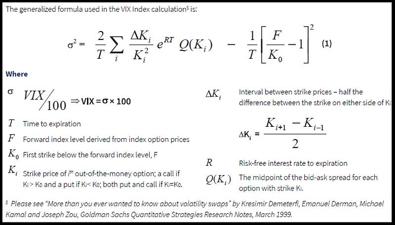
📌 How It Works in Python

A simplified version of calculating VIX using implied volatility from options data:

from scipy.stats import norm
import numpy as np


# Black-Scholes Implied Volatility Function
def black_scholes_iv(S, K, T, r, option_price, call=True):
    sigma = 0.2  # Initial guess
    for _ in range(100):
        d1 = (np.log(S / K) + (r + 0.5 * sigma ** 2) * T) / (sigma * np.sqrt(T))
        d2 = d1 - sigma * np.sqrt(T)
        if call:
            price = S * norm.cdf(d1) - K * np.exp(-r * T) * norm.cdf(d2)
        else:
            price = K * np.exp(-r * T) * norm.cdf(-d2) - S * norm.cdf(-d1)
        vega = S * norm.pdf(d1) * np.sqrt(T)
        sigma -= (price - option_price) / vega  # Newton-Raphson method
    return sigma
# Example: Find implied volatility for an S&P 500 option
iv = black_scholes_iv(S=4000, K=4100, T=0.25, r=0.02, option_price=200)
print("Implied Volatility:", iv)

This estimates implied volatility, a key input for VIX calculation.

GitHub repository of 15 Free Quant Trading Strategies in Python

Each strategy is designed for historical backtesting and forward testing, providing a solid foundation for building your own quant trading system.

🚀 Ready to dive in? Get the full repository here and start coding your own trading algorithms! 🚀

A Message from InsiderFinance

Thanks for being a part of our community! Before you go:

• 👏 Clap for the story and follow the author 👉

• 📰 View more content in the InsiderFinance Wire

• 📚 Take our FREE Masterclass

• 📈 Discover Powerful Trading Tools